Walmart dataset analysis - An in-depth analysis on sales across several states using Machine Learning
In this project, we cover some of the time series methods used in past competitions [7][8][9] to investigate the dataset provided by Walmart.
First, we build a special kind of RNN model called LSTM which attempts to predict the unit sales of individual stores. This is done by considering a univariate model and then using a more complex multivariate model, which we hope increases the test accuracy. Next, from the scikit-learn library in Python, we build an RF model which analyzes the item HOUSEHOLD_1_272_CA_3_validation, whilst selecting the most important features which help predict the sales of this particular product. We also compare the Random Forest (RF) results with other scikit-learn models. Lastly, we use an ARIMA model to predict the unit sales of the category HOBBIES whilst considering the fact that the dataset may not be stationary and pre-processing may be required before making progress.
Data Management:
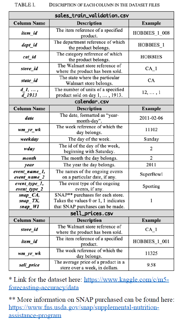
Walmart created the files for the M5 competition sales_train_validation.csv, calendar.csv and sell_prices.csv. The first contains the daily unit sales for a 3,049 products over the last 1,913 days and the date of the first day being 2011-01-29 and the last being 2016-06-19. Each product is categorized by one of 7 departments, 3 categories, 10 stores and 3 states. The second contains columns describing the dates and events for each day a product is sold. The last contains information regarding the price of each item for each store on a certain day.
Exploration:
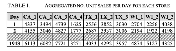
Our investigation for the RNN model began by looking at the number of unit sales per day for each Walmart store. We imported the dataset into Python as a pandas data frame. Then, we dropped the redundant columns from the original dataset and summed the unit sales per day and grouped them by store_id.
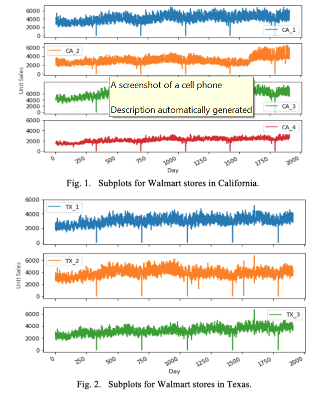
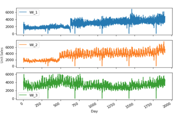
Next, we produced separate plots for stores based on the state they’re located in. The idea was to visually identify whether stores from the same state follow any obvious trend to justify univariate and multivariate models. We’d then go on to see whether introducing multiple variables has any significant impact on our predictions.
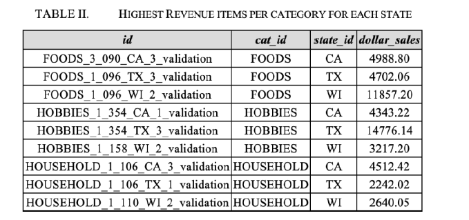
We also explored, for the RF model, the top 10 highest revenue items in Walmart stores for each category and state through the entire history of the dataset. As in Table III, the product FOODS_3_090_CA_3_validation is the most famous food item in CA with total dollar sales of $4988.90,
Subsequently, we looked at the time series prediction of HOUSEHOLD_1_272_CA_3_validation. We stored the daily sales of this item throughout the timeline in a data frame and transposed the matrix. Then, we joined this item to calendar.csv to get the details of events happening on each day which gave us flexibility in answering questions like why sales in one day was greater than another.
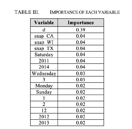
High loss is generally caused by models that are unable to learn from the training data. This means we have either used too few features such that the model is unable to map the data points causing under-fitting or the model is memorizing the mappings such that it may behave poorly on unseen data causing over-fitting. In our case, since we have around 60 features to train on, we’re likely to overfit. In Table III, we’ve created an importance table that allows us to see the importance of each variable in our dataset. The results suggest that variable 𝑑 is most important, representing the day, followed by snap_CA, snap_TX and snap_WI. The most important years were 2011, 2014 and the most important months were 3, 1 (March and January).
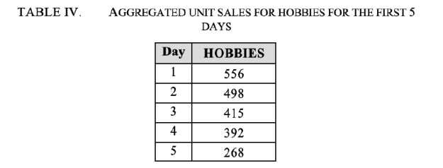
The goal for the ARIMA model was to predict the sales a store makes for products that belong to a specific category; in our case we base our focus on the HOBBIES category of CA_1. We started by loading the data into a pandas data frame and grouped our data by store and then by category. This was possible with the help of the pandas group_by function. Lastly, we added all the values for each day in each group.
Methodology:
- RNN:
We used RNNs in this project as they’re able to capture the patterns of multivariate input data which is suitable for the task we’re undertaking [1]. They can easily handle sequential data like ours and it considers the previously received inputs, unlike a typical Feed Forward neural network. We use TensorFlow with the Keras RNN API, which is designed for modelling sequential data for time series problems. We utilize a particular kind of RNN network called LSTM.
- RF:
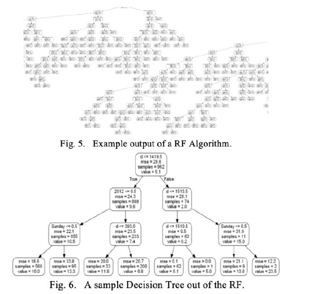
To complement the competence of RFs over other machine learning models as mentioned in Section III, we constructed a comparison chart evaluating the performance of scikit-learn models on our training and test sets. To make the predictions, we split 80% of the data for training on scikit-learn’s Random Forest Regressor. We used 1,000 estimators with random state set to zero. After fitting the model, we obtained an MAE of 5.85 on our test set. For simplicity, we’re representing just 3 layers of the tree.
- Arima:
that information in the past of a time series can be sufficient to accurately predict values in the future. The model has the general notation ARIMA(𝑝,𝑑,𝑞), where 𝑝 is the order of Auto Regressive term and refers to the number of time lags 𝑡 to be used as predictors, 𝑑 is the minimum number of differencing required to make a non-stationary series stationary and 𝑞 is the order of the Moving Average term indicating the required number of lagged forecast errors. It can be represented by the following equation: 𝜙(𝐿)(1−𝐿)𝑑𝑋𝑡=𝜇+𝛩(𝐿)𝜖𝑡, () where 𝜖𝑡 is the white noise distribution process 𝑊𝑁(0,𝜎2) and 𝐿 is the backward-shift operator with: 𝜙(𝐿)=1−𝜙1𝐿−⋯−𝜙𝑝𝐿𝑝, () 𝛩(𝐿)=1−𝛩1𝐿+⋯+𝛩𝑞𝐿𝑞, () with 𝜙𝑝,𝛩𝑞≠0.
Testing and Results:
- Univariate Model:
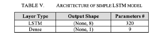
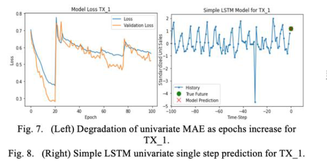
We introduce a simple LSTM model with a single 8-unit LSTM layer for a single-step prediction. We shuffle the tensors, cache the dataset and use batches of size 128 to propagate through the network so that training is faster and the memory requirement is less. We use a stochastic gradient descent optimizer which simply computes: 𝜃𝑡+1=𝜌𝜃𝑡−𝛼𝛻𝜃 where 𝜃 is the weight vector at a specified time, 𝑡 is the time being a certain day, 𝜌is the momentum which helps accelerate the gradient descent process to achieve faster convergence, 𝛼 is the LR of the optimizer and 𝛻𝜃 is the gradient with given weights. Over 100 epochs, we train our model and experiment with the LR using values 0.01 and 0.05.
It’s common practice to rescale the dataset before training a neural network [16] to help avoid the problem of getting stuck at local optima.The loss function we use is MAE. We see the best prediction for the univariate single-step model come from store TX_1 with LR 0.05.
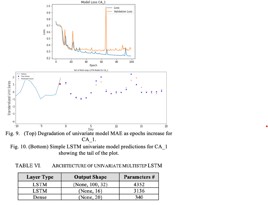
We also introduce multiple steps into the univariate time series where we attempt to predict 20 future steps. Since this is a more complex task, we add a 16-unit LSTM layer, with the original LSTM layer increased to 32 and the dense layer to 20. We see the best prediction comes from CA_1 and with LR 0.05.
- Multivariate Model:
A) LSTM:
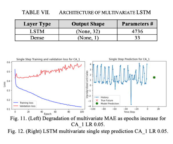
Since the multivariate task is a higher order of complexity, for the single-step model, we increase the number of units in the LSTM from 8 to 32. All other parameters of the model remain, with the only experimental adjustment being the LR. When doing the multivariate prediction for a store, we only use the data in stores which belong in the same state, meaning when we make a prediction on the unit sales of TX_1, we only consider the data in stores TX_1, TX_2 and TX_3. For the multivariate, multistep model, we adopt the same architecture as the single-step.
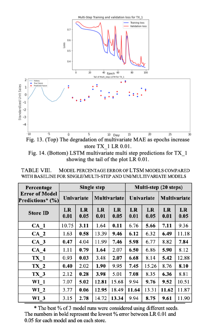
From the results in Table VIII, we find for the multi-step models that decreasing the LR generally leads to improvement in predictive performance on each store. It is unclear whether this improvement exists with the single-step models. In fact, the univariate model favors the higher LR. We see in the single-step case, for 9 out of 10 stores, the univariate model achieves the lowest percentage error (over LR 0.01 or 0.05) than the multivariate model, which may mean we’re overcomplicating matters by fitting redundant features. This cannot be said for the multi-step case, where 5 out of 10 stores for the multivariate model perform better than their univariate counterpart. This leads us to believe that for multi-step, for some stores, we under-fit the data by oversimplying the problem using a univariate model but we manage to capture the trend of the data better by using a more complex multivariate model.
B) Random Forest:
We set a threshold of 0.2, so that the variables which have importance factors greater than 0.2 will be considered for analysis as in Table III. We analysed the item HOUSEHOLD_1_272_CA_3_validation and when we fitted our model, we realized that reducing the number of features had a bad impact on our MAE, causing it to increase to 11.44.

To improve our results, we used several techniques: Data Scaling: The input features were scaled using Sklearn with the MAE being 8.49 after fitting the model and calculating predictive labels. Feature Selection. To increase the performance, we chose another group of features now with “snap_CA”, “snap_TX”, “snap_WI”, “Chanukah End”, “Christmas”, “Columbus Day”,” LentStart,” ,“VeteransDay”, “Day of the week”, “month” and “year”. The month, year and day of the week were all one-hot encoded. Test Split Sizes.
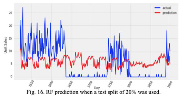
a. Test Split 20%
The data frame we obtained after feature selection step had 35 columns. The test size was set to 20%, so that 80 % of the data should be used for training. We saw a decrease of the MAE to 5.94.
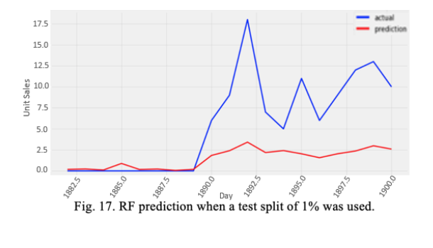
b. Test Split 1%:
Here, we took a test split of 0.01, meaning that 99% of the data would be used for training. The result obtained was far better than the previous case with test MAE of 4.33. The results indicate that, with greater test split, we’re compromising on our training quality since less data is available for training. This is shown through the decrease of the MAE when we decreased the test split.
Comparing with other Scikit Models. We were aware that other models in scikit-learn could potentially perform better than RF. To check this, we evaluated the performance of all models in scikit-learn library against our data as in Table IX.
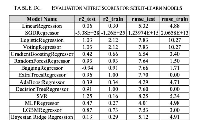
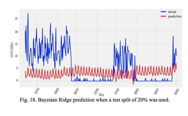
Bayesian Ridge Regression (BRR). It’s evident that BRR is one of the best performing models. To further understand how this model performs on our dataset, we decided to visualize its performance on different test splits.
a. Test Split 20%: Using BRR with a test split of 0.2, we obtain an MAE of 5.84.
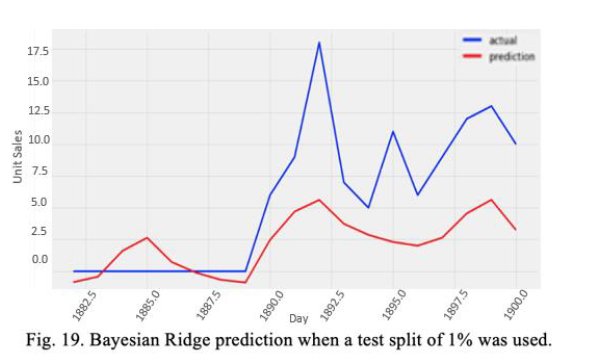
b. Test Split 1%
Now, using a test split of 0.01, our results are better. We obtain an MAE of 3.90 which is a significant performance increase compared with the same split for the RF prediction.
Experiments clearly show that BRR and RFs both need more data for reliable predictions. If we try to increase the test split, this will give the model less data to train on, making the predictive performance worse but having a higher certainty of it. If we decrease the test split, we’ll get a better prediction due to more training data but higher variance results for unseen data.
C. ARIMA:
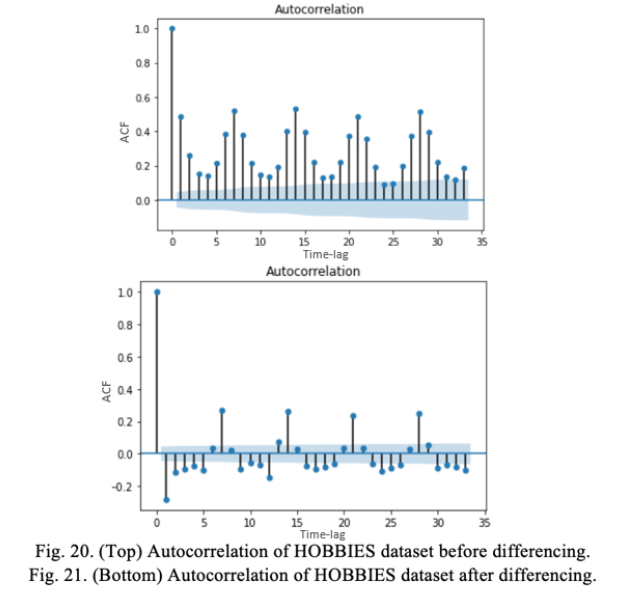
We first checked whether the dataset was in fact stationary. In Fig. 20, we found that it wasn’t stationary since the bars after time-lag 0 don’t lie within the critical interval. To fix this, we used differencing and depending on the complexity of the series, it may be needed more than once, as in Fig. 21. We made use of a built-in function called diff and were able to implement our ARIMA model to make some predictions.
We then use the ARIMA function that comes with the statsmodels.tsa.arima_model package. We used only 365 days of historic data, since ARIMA models tend to perform better in shorter timeframes. We split the 365 days into training and testing sets, approximately 90% and 10% respectively. To train the model, we send the train data as a parameter and specify each parameter required for the ARIMA(𝑝,𝑑,𝑞) model. After this, we fit our model by calling the fit function on our trained model. To make predictions, we call the function forecast on our fitted model and specify the number of predictions we want to make. In our case, we set that number to 24 with our prediction shifted to better fit the data.
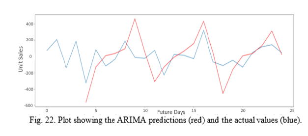
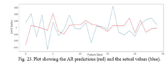
We observe that our model is able to capture the pattern of the data to some extent. The MSE obtained with this approach was 239.97. So, we decided to implement another model that works in a similar way to see if we could lower that value. We opted for the autoregressive (AR) model. The process is similar to the ARIMA model with the only difference being the training of the model. We use the AR function instead and we only send the training data as a parameter. Again, we fit our model and finally we make predictions by calling the predict function on the fitted model.
Limitations: We found that with building deeper RNNs, computational complexity increases and therefore so does training time or the resources required. ARIMA required a fair amount of preprocessing of the data in order to eventually build a model fit for training, specifically with differencing to ensure the model is stationary. We found with RF, finding the best split for reliable training yet good test accuracy proved to be a challenge.
Future work. If we could do further analysis, we would utilize Google’s TPUs further to build a deeper, more complex RNN model since time-series forecasting is not a simple task. It’s unclear from our results that introducing a more complex multivariate model improves the performance. It would be interesting to see if a more complex model than the one we implemented would improve performance. However, a deep model isn’t necessarily a better one [10]. Moreover, we could’ve tried a hybrid model, as Smyl in the M4 competition “which blended exponential smoothing and ML concepts into a single model of remarkable accuracy” [9] In the M4 competition paper, discussed is the “best model versus combining against single methods” where Makridakis et al. consistently find higher accuracy from combining than from a single model. Combining methods together produces diversity within a model, which helps cancel out random noise, thus leading to improved performance. Hence, combining RF, ARIMA and RNN could lead to even better results.
REFERENCES: [1] H.Hewamalage et al., “Recurrent Neural Networks for Time Series Forecasting: Current Status and Future Directions.” [2] S.Hochreiter et al., “Flat Minima,” LONG SHORT-TERM MEMORY, Jan.1997. [3] A.Hunt et al., The pragmatic programmer: from journeyman to master. Boston:Addison-Wesley, 2015. [4] M.J.Kane et al., “Comparison of ARIMA and Random Forest time series models for prediction of avian influenza H5N1 outbreaks,” BMC Bioinformatics, Aug.2014. [5] Y.LeCun et al., “Deep learning,” Nature, May.2015. [6] S.Makridakis et al., “The accuracy of extrapolation (time series) methods: Results of a forecasting competition,” Journal of Forecasting, Apr.1982. [7] S.Makridakis et al., “The M2-competition: A real-time judgmentally based forecasting study,” International Journal of Forecasting, Apr.1993. [8] S.Makridakis et al., “The M3-Competition: results, conclusions and implications,” International Journal of Forecasting, 2000. [9] S.Makridakis et al., “The M4 Competition: 100,000 time series and 61 forecasting methods,” International Journal of Forecasting, Jan.2020. [10] E.Malach et al., “Is Deeper Better only when Shallow is Good?,” Mar.2019. [11] J.N.K.Rao et al., “Time Series Analysis Forecasting and Control,” Sep.1972. [12] A.Redd et al., “Fast ES-RNN: A GPU Implementation of the ES-RNN Algorithm.” [13] V.Svetnik, et al., “Random Forest: A Classification and Regression Tool for Compound Classification and QSAR Modeling,” Journal of Chemical Information and Computer Sciences, Nov.2003. [14] Y.Takefuji et al., “Effectiveness of ensemble machine learning over the conventional multivariable linear regression models,” Jan.2016. [15] H.Tanaka, “Fuzzy data analysis by possibilistic linear models,” Fuzzy Sets and Systems, Dec.1987. [16] W.Williams et al., “SCALING RECURRENT NEURAL NETWORK LANGUAGE MODELS.”
Code Implementation We used notebooks to create our well-documented codes so that it is easy for the reader to follow. They were used to generate the results for each model and can be found on our GitHub repository: https://github.com/GerardoMoreno96/ECS784P_DataAnalyticsProject
Dataset: